- (*)Gaussian probability density function:
Write a function gaussian.m that can compute the Gaussian probability density function, with the following usage:
The input and output arguments are:
out = gaussian(data, mu, sigma); - data: a data matrix of size d by n, representing n data vectors, each with dimension d.
- mu: a mean vector of dimension d by 1.
- sigma: a covariance matrix of dimension d by d.
- out: an output vector of syze 1 by n.
Solution: Please refer to SAP Toolbox. - (*)MLE of a Gaussian PDF:
Write a function gaussianMle.m to compute the MLE of a Gaussian PDF, with the following usage:
The input and output arguments are:
[mu, sigma] = gaussianMle(data); - data: a data matrix of size d by n, representing n data vectors, each with dimension d.
- mu: a mean vector of dimension d by 1.
- sigma: a covariance matrix of dimension d by d.
Solution: Please refer to SAP Toolbox. - (*)MLE of Gaussian for 1D data:
Please use the above functions (gaussian.m and gaussianMle.m) to accomplish the following tasks:
- Assume the 1D data is generated by the following code:
dataNum=1000; data = randn(1, dataNum); - Use gaussianMle.m to find the optimum mu and sigma.
- Use gaussian.m to plot the Gaussian PDF using the obtained mu and sigma.
- Use hist.m to plot the histogram. Please adjust the bin number such that the histogram has a shape close to that of the Gaussian function. What the best bin number in your experiment?
- In fact, you need to multiply the Gaussian function by a constant k such that the it can approximate the histogram. Please derive the value of the constant k. What is the value of k in this exercise?
- Assume the 1D data is generated by the following code:
- (*)MLE of Gaussian for 2D data:
Repeat the previous exercise using 2D data generated by the following code:
(Hint: You need to write your own hist.m for 2D data.)
dataNum=1000; x=randn(1, dataNum); y=randn(1, dataNum)/2; data=[x; x+y]; plot(data(1, :), data(2,:), '.'); - (**)GMM evaluation:
Write a function gmmEval.m to compute GMM with the following usage:
The input and output arguments are:
out = gmmEval(data, mu, sigma, w); - data: a data matrix of dimension d by n, where there are n data vectors, each with dimension d by 1.
- mu: a mean matrix of dimension d by m, where there are m mean vectors, each with dimension d by 1.
- sigma: a vector of size 1 by m, where sigma(i)*eye(d) is the covariance matrix for mixture i.
- w: a vector of size 1 by m, where w(i) is the weighting factor of mixture i. The summation of w is 1.
- out: a output vector of 1 by n.
- (***)GMM training:
Write a function gmmTrain.m to perform the training of a GMM, with the usage:
The input and output arguments are:
[mu, sigma, w, logProb] = gmmTrain(data, m) - data: a data matrix of dimension d by n, where there are n data vectors, each with dimension d by 1.
- m: number of mixture in the GMM
- mu: a mean matrix of dimension d by m, where there are m mean vectors, each with dimension d by 1.
- sigma: a vector of size 1 by m, where sigma(i)*eye(d) is the covariance matrix for mixture i.
- w: a vector of size 1 by m, where w(i) is the weighting factor of mixture i. The summation of w is 1.
- out: a output vector of 1 by n.
- (*)MLE of GMM for 1D data:
Use the functions (gmmEval.m and gmmTrain.m) in the SAP toolbox to accomplish the tasks:
- Assume the 1D data is generated by the following code:
dataNum = 100; data1 = randn(1,2*dataNum); data2 = randn(1,3*dataNum)/2+3; data3 = randn(1,1*dataNum)/3-3; data4 = randn(1,1*dataNum)+6; data = [data1, data2, data3, data4]; - Use hist.m to plot the histogram of the data set. Please adjust the bin number such that the histogram is able to show the distribution in an appropriate manner.(Hint: use hist(data, binNum) to plot the histogram.)
- Assume the number of mixture is 4 and use gmmTrain.m to find the best mu, sigma, and w.
- Use gmmEval.m to plot the GMM function using the obtained parameters. If the curve of the GMM does not look similar to the histogram, please increase gmmOpt.train.maxIteration. (Hint: The output of gmmEval.m is log probability density (also known as log likelihood); you need to transform it back to common probability density.)
- In fact, you need to multiply the Gaussian function by a constant k such that the it can approximate the histogram. Please derive the value of the constant k. What is the value of k in this exercise?
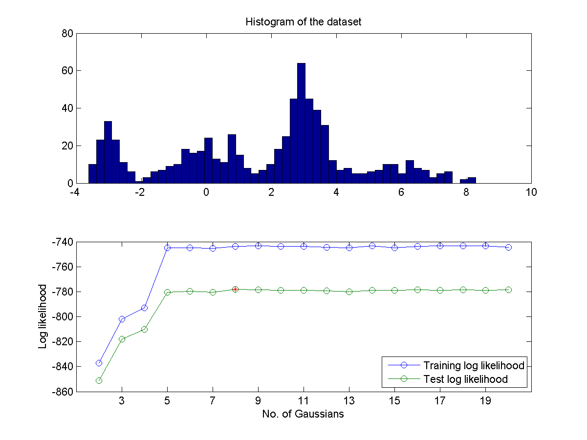
- If you do not know the number of mixture in advance, can you find a way to identify the best number of mixture? One way to do this is to partition the data into two sets A and B. Use set A for training GMM and set B for validation. Then plot the log likelihood of both A and B as a functions of the numbers of Gaussians. Then you can determine the optimum number of Gaussians is the one that can achieve the maximum of log likelihood in set B. A typical plot is shown next:
- As can be imagined, the above method for determining the optimum number of Gaussians is highly affected by the way we partition the dataset. A more robust method is based on the leave-one-out criterion which takes full advantage of the whole dataset. Use such a method to obtain a similar plot shown in the previous exercise. Does the identified optimum Gaussian number more reliable? Why or why not.
- Assume the 1D data is generated by the following code:
- (*)MLE of GMM for 2D data:
Repeat the previous exercise using 2D data generated by the following code:
In (a), you should set the number of mixtures to 8. (Hint: You need to write your own hist.m for 2D data.)
DS = dcData(6); dsScatterPlot(DS); - (**)Two-fold cross validation of GMM on IRIS dataset: Please repeat the example, but using 2-fold cross validation to compute the recognition rates.
- (**)Leave-one-out test of GMM on IRIS dataset: Please repeat the example, but using the leave-one-out test fo compute the recognition rates.
- (**)Two-fold cross validation of GMM on IRIS dataset, with varying numbers of mixtures:
Please repeat the example, but using 2-fold cross validation to compute the recognition rates. Note that:
- You should demonstrate two curves representing the inside-test and out-side test recognition rates. The obtained curves should be smoother than those shown in the example.
- If the data size is too small for a certain iteration, you can reduce the number of mixtures accordingly.
- (**)Leave-one-out test of GMM on IRIS dataset, with varying numbers of mixtures:
Please repeat the example, but using the leave-one-out test to compute the recognition rates. Note that:
- You should demonstrate two curves representing the inside-test and out-side test recognition rates. The obtained curves should be smoother than those shown in the example.
- If the data size is too small for a certain iteration, you can reduce the number of mixtures accordingly.
- (**)Leave-one-out test of GMM on WINE dataset, with varying numbers of mixtures:
Repeat the example, but using the leave-one-out test to compute the recognition rates. Note that you should have two plots (corresponding to the following conditions), each with two curves of the inside-test and out-side test recognition rates.
- Without input normalization.
- With input normalization.
- (**)Leave-one-out test of GMM on vowel dataset, with varying numbers of mixtures: Repeat the previous exercise using the data in the exercise "Use MFCC for classifying vowels"
Data Clustering and Pattern Recognition (資料分群與樣式辨認)
